Warning
This page was created from a pull request (#70).
Portfolio selection
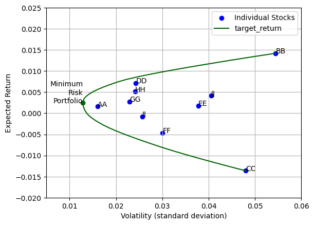
Given a sum of money to invest, one must decide how to spend it amongst a portfolio of financial securities. Our approach is due to Markowitz (1959) and looks to minimize the risk associated with the investment while realizing a target expected return. By varying the target, one can compute an ‘efficient frontier’, which defines the optimal portfolio for a given expected return.
Adapted from the Gurobi examples. This does not illustrate the accessor API since all constraints are single expressions.
Point to think about though: when we do construct a single expression by applying pandas operations to series, the user has to fall back onto gurobipy methods.
[1]:
import gurobipy as gp
from gurobipy import GRB
from math import sqrt
import gurobipy_pandas as gppd
import pandas as pd
import numpy as np
import matplotlib
import matplotlib.pyplot as plt
Import (normalized) historical return data using pandas
[2]:
data = pd.read_csv('data/portfolio.csv', index_col=0)
Create a new model and add a variable for each stock. The columns in our dataframe correspond to stocks, so the columns can be used directly (as a pandas index) to construct the necessary variable.
[3]:
model = gp.Model('Portfolio')
stocks = gppd.add_vars(model, data.columns, name="Stock")
model.update()
stocks
Restricted license - for non-production use only - expires 2025-11-24
[3]:
AA    <gurobi.Var Stock[AA]>
BB    <gurobi.Var Stock[BB]>
CC    <gurobi.Var Stock[CC]>
DD    <gurobi.Var Stock[DD]>
EE    <gurobi.Var Stock[EE]>
FF    <gurobi.Var Stock[FF]>
GG    <gurobi.Var Stock[GG]>
HH    <gurobi.Var Stock[HH]>
II    <gurobi.Var Stock[II]>
JJ    <gurobi.Var Stock[JJ]>
Name: Stock, dtype: object
Objective is to minimize risk (squared). This is modeled using the covariance matrix, which measures the historical correlation between stocks.
[4]:
sigma = data.cov()
portfolio_risk = sigma.dot(stocks).dot(stocks)
model.setObjective(portfolio_risk, GRB.MINIMIZE)
Fix budget with a constraint. For summation over series, we get back just a single expression, so this constraint is added directly to the model (not through the accessors).
[5]:
model.addConstr(stocks.sum() == 1, name='budget');
Optimize model to find the minimum risk portfolio.
[6]:
model.optimize()
Gurobi Optimizer version 11.0.0 build v11.0.0rc2 (linux64 - "Ubuntu 20.04.6 LTS")
CPU model: Intel(R) Xeon(R) Platinum 8259CL CPU @ 2.50GHz, instruction set [SSE2|AVX|AVX2|AVX512]
Thread count: 1 physical cores, 2 logical processors, using up to 2 threads
Optimize a model with 1 rows, 10 columns and 10 nonzeros
Model fingerprint: 0x9181cbde
Model has 55 quadratic objective terms
Coefficient statistics:
Matrix range [1e+00, 1e+00]
Objective range [0e+00, 0e+00]
QObjective range [3e-05, 7e-03]
Bounds range [0e+00, 0e+00]
RHS range [1e+00, 1e+00]
Presolve time: 0.01s
Presolved: 1 rows, 10 columns, 10 nonzeros
Presolved model has 55 quadratic objective terms
Ordering time: 0.00s
Barrier statistics:
Free vars : 9
AA' NZ : 4.500e+01
Factor NZ : 5.500e+01
Factor Ops : 3.850e+02 (less than 1 second per iteration)
Threads : 1
Objective Residual
Iter Primal Dual Primal Dual Compl Time
0 4.16767507e+03 -4.16767507e+03 1.00e+04 8.08e-06 1.00e+06 0s
1 4.45599962e-03 -7.80471122e+00 1.09e+01 8.83e-09 1.14e+03 0s
2 4.17460816e-04 -7.14114851e+00 1.09e-05 8.84e-15 4.57e+01 0s
3 4.17365279e-04 -7.33725047e-03 9.40e-10 2.78e-17 4.96e-02 0s
4 3.50058972e-04 -1.09469258e-04 2.26e-11 1.39e-17 2.94e-03 0s
5 1.95819453e-04 5.77538068e-05 2.22e-16 2.69e-17 8.84e-04 0s
6 1.72155801e-04 1.57430436e-04 5.55e-17 6.94e-18 9.42e-05 0s
7 1.66577780e-04 1.65061129e-04 6.66e-16 1.57e-17 9.71e-06 0s
8 1.65913497e-04 1.65828685e-04 1.67e-16 1.39e-17 5.43e-07 0s
9 1.65877870e-04 1.65873375e-04 5.41e-16 1.85e-18 2.88e-08 0s
10 1.65877097e-04 1.65877052e-04 3.39e-15 1.39e-17 2.88e-10 0s
Barrier solved model in 10 iterations and 0.03 seconds (0.00 work units)
Optimal objective 1.65877097e-04
Display the minimum risk portfolio.
[7]:
stocks.gppd.X.round(3)
[7]:
AA    0.468
BB    0.000
CC    0.003
DD    0.125
EE    0.000
FF    0.033
GG    0.017
HH    0.205
II    0.149
JJ    0.000
Name: Stock, dtype: float64
Key metrics
[8]:
minrisk_volatility = sqrt(portfolio_risk.getValue())
print('\nVolatility      = %g' % minrisk_volatility)

stock_return = data.mean()
portfolio_return = stock_return.dot(stocks)
minrisk_return = portfolio_return.getValue()
print('Expected Return = %g' % minrisk_return)
Volatility      = 0.0128793
Expected Return = 0.00243537
Solve for the efficient frontier by varying the target return (sampling).
One useful point here could be the ability to specify scenarios by mapping onto constraints
[9]:
scenarios = pd.DataFrame(dict(target_return=np.linspace(stock_return.min(), stock_return.max())))
target_return = model.addConstr(portfolio_return == minrisk_return, 'target_return')

model.update()

model.NumScenarios = len(scenarios)
for row in scenarios.itertuples():
    model.Params.ScenarioNumber = row.Index
    target_return.ScenNRHS = row.target_return

model.Params.OutputFlag = 0
model.optimize()

results = []
for row in scenarios.itertuples():
    model.Params.ScenarioNumber = row.Index
    results.append(model.ScenNObjVal)

scenarios = scenarios.assign(ObjVal=pd.Series(results, index=scenarios.index))

scenarios['volatility'] = scenarios['ObjVal'].apply(sqrt)
scenarios.head()
[9]:
| target_return | ObjVal | volatility | |
|---|---|---|---|
| 0 | -0.013629 | 0.002303 | 0.047985 |
| 1 | -0.013061 | 0.002114 | 0.045981 |
| 2 | -0.012492 | 0.001937 | 0.044008 |
| 3 | -0.011924 | 0.001769 | 0.042059 |
| 4 | -0.011356 | 0.001611 | 0.040140 |
[10]:
# Plot volatility versus expected return for individual stocks
stock_volatility = data.std()
ax = plt.gca()
ax.scatter(x=stock_volatility, y=stock_return,
           color='Blue', label='Individual Stocks')
for i, stock in enumerate(stocks.index):
    ax.annotate(stock, (stock_volatility[i], stock_return[i]))

# Plot volatility versus expected return for minimum risk portfolio
ax.scatter(x=minrisk_volatility, y=minrisk_return, color='DarkGreen')
ax.annotate('Minimum\nRisk\nPortfolio', (minrisk_volatility, minrisk_return),
            horizontalalignment='right')

# Plot efficient frontier
scenarios.plot.line(x='volatility', y='target_return', ax=ax, color='DarkGreen')

# Format and display the final plot
ax.axis([0.005, 0.06, -0.02, 0.025])
ax.set_xlabel('Volatility (standard deviation)')
ax.set_ylabel('Expected Return')
ax.legend()
ax.grid()